don’t be plastic, elastipy!

Hi there, this tutorial is actually a jupyter notebook and can be found in examples/tutorial.ipynb

exporting some objects

Without too much thinking we can just use the built-in export helper and generate some data.

from elastipy import Exporter

class ShapeExporter(Exporter):
    INDEX_NAME = "elastipy-example-shapes"
    MAPPINGS = {
        "properties": {
            "shape": {"type": "keyword"},
            "color": {"type": "keyword"},
            "area": {"type": "float"},
        }
    }

The INDEX_NAME is obviously the name of the elasticsearch index. The MAPPINGS parameter describes the elasticsearch mapping. Here we say that documents will at least have these common fields, one of type float and two of type keyword which means they are strings but not full-text searchable ones. Instead they are efficiently indexed and aggregatable.

The data we create out of thin air..

import random

def shape_generator(count=1000, seed=42):
    rnd = random.Random(seed)
    for i in range(count):
        yield {
            "shape": rnd.choice(("triangle", "square")),
            "color": rnd.choice(("red", "green", "blue")),
            "area": rnd.gauss(5, 1.3),
        }

Now create our exporter and export a couple of documents. It uses the bulk helper tools internally.

exporter = ShapeExporter()

count, errors = exporter.export_list(shape_generator(), refresh=True)

print(count, "exported")

1000 exported

The refresh=True parameter will refresh the index as soon as everything is exported, so we do not have to wait for objects to appear in the elasticsearch index.

query oh elastipyia

In most cases this import is enough to access all the good stuff:

from elastipy import Search, query

Now get some documents:

s = Search(index="elastipy-example-shapes")

s is now a search request that can be configured. Setting any search related options will always return a new instance. Here we set the maximum number of documents to respond:

s = s.size(3)

Next we add a query, more specifically a term query.

s = s.term(field="color", value="green")

Our request to elasticsearch would look like this right now:

s.dump.body()

{
  "query": {
    "term": {
      "color": {
        "value": "green"
      }
    }
  },
  "size": 3
}

More queries can be added, which defaults to an AND combination:

s = s.range(field="area", gt=5.)
s.dump.body()

{
  "query": {
    "bool": {
      "must": [
        {
          "term": {
            "color": {
              "value": "green"
            }
          }
        },
        {
          "range": {
            "area": {
              "gt": 5.0
            }
          }
        }
      ]
    }
  },
  "size": 3
}

OR combinations can be archived with the bool query itself or by applying the | operator to the query classes in elastipy.query:

s = s | (query.Term(field="color", value="red") & query.Range(field="area", gt=8.))
s.dump.body()

{
  "query": {
    "bool": {
      "should": [
        {
          "bool": {
            "must": [
              {
                "term": {
                  "color": {
                    "value": "green"
                  }
                }
              },
              {
                "range": {
                  "area": {
                    "gt": 5.0
                  }
                }
              }
            ]
          }
        },
        {
          "bool": {
            "must": [
              {
                "term": {
                  "color": {
                    "value": "red"
                  }
                }
              },
              {
                "range": {
                  "area": {
                    "gt": 8.0
                  }
                }
              }
            ]
          }
        }
      ]
    }
  },
  "size": 3
}

Better execute the search now before the body get’s too complicated:

response = s.execute()
response.dump()

{
  "took": 8,
  "timed_out": false,
  "_shards": {
    "total": 1,
    "successful": 1,
    "skipped": 0,
    "failed": 0
  },
  "hits": {
    "total": {
      "value": 185,
      "relation": "eq"
    },
    "max_score": 2.1868048,
    "hits": [
      {
        "_index": "elastipy-example-shapes",
        "_type": "_doc",
        "_id": "1Lf0jHcBB26LJVfaIvox",
        "_score": 2.1868048,
        "_source": {
          "shape": "square",
          "color": "red",
          "area": 9.422362274394294
        }
      },
      {
        "_index": "elastipy-example-shapes",
        "_type": "_doc",
        "_id": "FLf0jHcBB26LJVfaIvsx",
        "_score": 2.1868048,
        "_source": {
          "shape": "triangle",
          "color": "red",
          "area": 8.011022752102972
        }
      },
      {
        "_index": "elastipy-example-shapes",
        "_type": "_doc",
        "_id": "OLf0jHcBB26LJVfaIvsx",
        "_score": 2.1868048,
        "_source": {
          "shape": "square",
          "color": "red",
          "area": 8.001834685241512
        }
      }
    ]
  }
}

The response object is a small wrapper around dict that has some convenience properties.

response.documents

[{'shape': 'square', 'color': 'red', 'area': 9.422362274394294},
 {'shape': 'triangle', 'color': 'red', 'area': 8.011022752102972},
 {'shape': 'square', 'color': 'red', 'area': 8.001834685241512}]

How many documents are there at all?

Search(index="elastipy-example-shapes").execute().total_hits

The functions and properties are tried to make chainable in a way that allows for short and powerful oneliners:

Search(index="elastipy-example-shapes") \
    .size(20).sort("-area").execute().documents

[{'shape': 'triangle', 'color': 'red', 'area': 10.609408732815844},
 {'shape': 'square', 'color': 'blue', 'area': 9.785991184126697},
 {'shape': 'square', 'color': 'red', 'area': 9.422362274394294},
 {'shape': 'triangle', 'color': 'blue', 'area': 9.24591971667655},
 {'shape': 'square', 'color': 'blue', 'area': 9.11442473191995},
 {'shape': 'square', 'color': 'green', 'area': 8.928816107277179},
 {'shape': 'square', 'color': 'blue', 'area': 8.473742067630953},
 {'shape': 'triangle', 'color': 'green', 'area': 8.128635913090859},
 {'shape': 'triangle', 'color': 'blue', 'area': 8.033908240900079},
 {'shape': 'square', 'color': 'green', 'area': 8.030514737232895},
 {'shape': 'triangle', 'color': 'red', 'area': 8.011022752102972},
 {'shape': 'square', 'color': 'red', 'area': 8.001834685241512},
 {'shape': 'square', 'color': 'green', 'area': 7.986094071679083},
 {'shape': 'square', 'color': 'blue', 'area': 7.984604837392737},
 {'shape': 'triangle', 'color': 'blue', 'area': 7.965890845028483},
 {'shape': 'square', 'color': 'green', 'area': 7.937110248587943},
 {'shape': 'square', 'color': 'blue', 'area': 7.933212484940288},
 {'shape': 'triangle', 'color': 'blue', 'area': 7.900062931477738},
 {'shape': 'square', 'color': 'green', 'area': 7.892344075058484},
 {'shape': 'triangle', 'color': 'blue', 'area': 7.883278182699227}]

So that was rambling about the filtering and the documents in the response. There is a lot of functionality in elasticsearch that is not covered by this library right now. To move on in happiness we just start the next chapter.

agitated aggregation

Aggregations can be created using the agg_, metric_ and pipeline_ prefixes. An aggregation is attached to the Search instance, so there is no copying like with the queries above.

s = Search(index="elastipy-example-shapes").size(0)

agg = s.agg_terms(field="shape")

s.dump.body()

{
  "aggregations": {
    "a0": {
      "terms": {
        "field": "shape"
      }
    }
  },
  "query": {
    "match_all": {}
  },
  "size": 0
}

As we can see, a terms aggregation has been added to the search body. The names of aggregations are auto-generated, but can be explicitly stated:

s = Search(index="elastipy-example-shapes").size(0)

agg = s.agg_terms("shapes", field="shape")

s.dump.body()

{
  "aggregations": {
    "shapes": {
      "terms": {
        "field": "shape"
      }
    }
  },
  "query": {
    "match_all": {}
  },
  "size": 0
}

Let’s look at the result from elasticsearch:

s.execute().dump()

{
  "took": 2,
  "timed_out": false,
  "_shards": {
    "total": 1,
    "successful": 1,
    "skipped": 0,
    "failed": 0
  },
  "hits": {
    "total": {
      "value": 1000,
      "relation": "eq"
    },
    "max_score": null,
    "hits": []
  },
  "aggregations": {
    "shapes": {
      "doc_count_error_upper_bound": 0,
      "sum_other_doc_count": 0,
      "buckets": [
        {
          "key": "square",
          "doc_count": 513
        },
        {
          "key": "triangle",
          "doc_count": 487
        }
      ]
    }
  }
}

valuable access

Because we kept the agg variable, we can use it’s interface to access the values more conveniently:

agg.to_dict()

{'square': 513, 'triangle': 487}

It supports the items(), keys() and values() generators as known from the dict type:

for key, value in agg.items():
    print(f"{key:12} {value}")

square       513
triangle     487

It also has a dict_rows() generator which preserves the names and keys of the aggregations:

for row in agg.dict_rows():
    print(row)

{'shapes': 'square', 'shapes.doc_count': 513}
{'shapes': 'triangle', 'shapes.doc_count': 487}

The rows() generator flattens the dict_rows() into a CSV-style list:

for row in agg.rows():
    print(row)

['shapes', 'shapes.doc_count']
['square', 513]
['triangle', 487]

And we can print a nice table to the command-line:

agg.dump.table(colors=False)

shapes   │ shapes.doc_count
─────────┼────────────────────────────────────────────
square   │ 513 ███████████████████████████████████████
triangle │ 487 █████████████████████████████████████

(The colors=False parameter disables console colors because they do not work in this documentation)

Obviously, at this point a couple of users would not understand why there is no conversion to a pandas DataFrame built in:

agg.to_pandas()  # or simply agg.df()

	shapes	shapes.doc_count
0	square	513
1	triangle	487

The columns are assigned automatically.

Columns containing ISO-formatted date strings will be converted to pandas.Timestamp.

The DataFrame index column can be assigned with the index and to_index parameters.

index simply copies the column:

agg.to_pandas(index="shapes")

	shapes	shapes.doc_count
shapes
square	square	513
triangle	triangle	487

to_index will move the column:

agg.to_pandas(to_index="shapes")

	shapes.doc_count
shapes
square	513
triangle	487

With matplotlib installed we can access the pandas plotting interface:

agg.df(to_index="shapes").plot.bar()

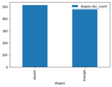
Satisfied with a little graphic we feel more confident and look into the details of metrics and nested bucket aggregations.

deeper aggregation agitation

agg = Search(index="elastipy-example-shapes") \
    .agg_terms("shapes", field="shape") \
    .agg_terms("colors", field="color") \
    .metric_sum("area", field="area") \
    .metric_avg("area-avg", field="area") \
    .execute()

A few notes:

agg_ methods always return the newly created aggregation, so the colors aggregation is nested inside the shapes aggregation.
metric_ methods return their parent aggregation (because metrics do not allow a nested aggregation), so we can just continue to call metric_* and each time we add a metric to the colors aggregation. If you need to get access to the metric object itself add the return_self=True parameter.
The execute method on an aggregation does not return the response but the aggregation itself.

Now, what does the to_dict output look like?

agg.to_dict()

{('square', 'blue'): 178,
 ('square', 'green'): 170,
 ('square', 'red'): 165,
 ('triangle', 'blue'): 177,
 ('triangle', 'green'): 170,
 ('triangle', 'red'): 140}

It has put the keys that lead to each value into tuples. Without a lot of thinking we can say:

data = agg.to_dict()
print(f"There are {data[('triangle', 'red')]} red triangles in the database!")

There are 140 red triangles in the database!

But where are the metrics gone?

Generally, keys(), values(), items(), to_dict() and to_matrix() only access the values of the current aggregation (which is colors in the example). Although all the keys of the parent bucket aggregations that lead to the values are included.

The methods dict_rows(), rows(), to_pandas() and .dump.table() will access all values from the whole aggregation branch. In this example the branch looks like this:

shapes
colors
- area
- area-avg

agg.dump.table(digits=3, colors=False)

shapes   │ shapes.doc_count    │ colors │ colors.doc_count    │ area                    │ area-avg
─────────┼─────────────────────┼────────┼─────────────────────┼─────────────────────────┼─────────────────────
square   │ 513 ███████████████ │ blue   │ 178 ███████████████ │ 920.602 ███████████████ │ 5.172 █████████████▉
square   │ 513 ███████████████ │ green  │ 170 ██████████████▍ │ 882.643 ██████████████▍ │ 5.192 ██████████████
square   │ 513 ███████████████ │ red    │ 165 █████████████▉  │ 848.229 █████████████▉  │ 5.141 █████████████▉
triangle │ 487 ██████████████▍ │ blue   │ 177 ██████████████▉ │ 891.198 ██████████████▌ │ 5.035 █████████████▋
triangle │ 487 ██████████████▍ │ green  │ 170 ██████████████▍ │ 834.699 █████████████▋  │  4.91 █████████████▍
triangle │ 487 ██████████████▍ │ red    │ 140 ███████████▉    │ 704.332 ███████████▋    │ 5.031 █████████████▋

Now all information is in the table. Note that the shapes.doc_count column contains the same value multiple times. This is because each colors aggregation bucket splits the shapes bucket into multiple results, without changing the overall count of the shapes, of course.

It’s possible to move the keys of sub-aggregations into new columns with the flat parameter. Below we basically say: Drop the colors and colors.doc_count columns and instead create a column for each encountered color key. The names of following sub-aggregations and metrics are appended to each key. (Also the resulting area-avg columns are excluded to not hurt our eyes too much)

agg.dump.table(flat="colors", exclude="*avg", digits=3, colors=False)

shapes   │ shapes.doc_count │ blue       │ blue.area      │ green │ green.area      │ red      │ red.area
─────────┼──────────────────┼────────────┼────────────────┼───────┼─────────────────┼──────────┼──────────────
square   │ 513 ████████████ │ 178 ██████ │ 920.602 ██████ │ 170   │ 882.643 ███████ │ 165 ████ │ 848.229 █████
triangle │ 487 ███████████▌ │ 177 █████▉ │ 891.198 █████▊ │ 170   │ 834.699 ██████▋ │ 140 ███▌ │ 704.332 ████▎

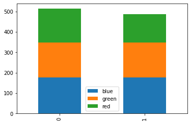
This can be useful for stacking bars in a plot:

agg.df(flat="colors", exclude=("*doc_count", "*area*")).plot.bar(stacked=True)

Now what is this method with the awesome name to_matrix?

names, keys, matrix = agg.to_matrix()
print("names ", names)
print("keys  ", keys)
print("matrix", matrix)

names  ['shapes', 'colors']
keys   [['square', 'triangle'], ['blue', 'green', 'red']]
matrix [[178, 170, 165], [177, 170, 140]]

It produces a heatmap! At least in two dimensions. In this example we have two dimensions from the bucket aggregations shapes and colors. to_matrix() will produce a matrix with any number of dimensions, but if it’s one or two, we can also convert it to a DataFrame:

agg.df_matrix()

	blue	green	red
square	178	170	165
triangle	177	170	140

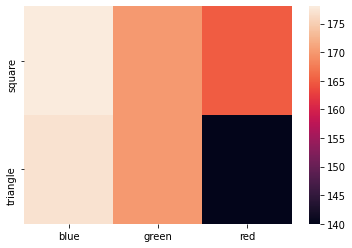
To access the values of metrics we have to call to_matrix on a metric aggregation. Our agg parameter contains the area and area-avg metrics and we can reach it with the children property. Below is the heatmap of the average area. Except for the values nothing changed because metrics (and pipelines) do not contribute to the keys.

agg.children[1].df_matrix()

	blue	green	red
square	5.171923	5.192018	5.140783
triangle	5.035015	4.909992	5.030943

Having something like seaborn installed we can easily plot it:

import seaborn as sns

sns.heatmap(agg.df_matrix())