Plotting maps

Here are examples to plot geographic data using plotly and matplotlib. Matplotlib is probably the choice if you need a rendered image. Plotly creates interactive plots and has a more modern interface.

To handle the different geo-types returned by elasticsearch we first look at conversion utilities. Skip it if you just want to see pretty images.

Coordinate conversion

A metric aggregation like geo_centroid already returns latitude and longitude values.

Bucket-aggregations like geotile_grid and geohash_grid return keys that can be mapped to geo-coordinates.

map-tiles

The geotile_grid aggregation uses map-tiles (wikipedia) as bucket keys. They represent zoom/x/y as seen below:

from elastipy import Search

s = Search(index="elastipy-example-car-accidents")

agg = s.agg_geotile_grid("tiles", field="location", precision=6)

agg.execute().to_dict()

{'6/33/21': 131436,
 '6/34/21': 36158,
 '6/33/20': 35218,
 '6/33/22': 32519,
 '6/34/22': 19237,
 '6/34/20': 13802}

To convert the keys to geo-coordinates we can use a helper function in elastipy:

from elastipy import geotile_to_lat_lon

{
    geotile_to_lat_lon(key): value
    for key, value in agg.items()
}

{(50.736455137010644, 8.4375): 131436,
 (50.736455137010644, 14.0625): 36158,
 (54.162433968067795, 8.4375): 35218,
 (47.04018214480665, 8.4375): 32519,
 (47.04018214480665, 14.0625): 19237,
 (54.162433968067795, 14.0625): 13802}

Becaue the tiles are actually areas the latitude and longitude just represent a single point within the area. The point can be defined as the offset parameter and defaults to (.5, .5) which is the center of the tile.

Here we print the top-left and bottom-right coordinates for each map-tile:

for key, value in agg.items():
    tl = geotile_to_lat_lon(key, offset=(0, 1))
    bl = geotile_to_lat_lon(key, offset=(1, 0))
    print(f"{tl} - {bl}: {value}")

(48.92249926375824, 5.625) - (52.48278022207821, 11.25): 131436
(48.92249926375824, 11.25) - (52.48278022207821, 16.875): 36158
(52.48278022207821, 5.625) - (55.77657301866769, 11.25): 35218
(45.08903556483103, 5.625) - (48.92249926375824, 11.25): 32519
(45.08903556483103, 11.25) - (48.92249926375824, 16.875): 19237
(52.48278022207821, 11.25) - (55.77657301866769, 16.875): 13802

geohash

The geohash_grid aggregation returns geohash (wikipedia) bucket keys.

from elastipy import Search

s = Search(index="elastipy-example-car-accidents")

agg = s.agg_geohash_grid("tiles", field="location", precision=2)

agg.execute().to_dict()

{'u1': 113676, 'u0': 85497, 'u3': 41653, 'u2': 27544}

The pygeohash package can be used to translate them:

import pygeohash

{
    pygeohash.decode(key): value
    for key, value in agg.items()
}

{(53.0, 6.0): 113676,
 (48.0, 6.0): 85497,
 (53.0, 17.0): 41653,
 (48.0, 17.0): 27544}

For convenience the pygeohash function is wrapped by elastipy.geohash_to_lat_lon.

plotly backend

The plotly python library enables creating browser-based plots in python. It supports a range of map plots. In particular the mapbox based plots are interesting because they use WebGL and render quite fast even for a large number of items.

geo-centroid

Let’s plot an overview of the german car accidents (included in elastipy examples).

s = Search(index="elastipy-example-car-accidents")
agg = s.agg_terms("city", field="city", size=10000)
agg = agg.metric_geo_centroid("location", field="location")

df = agg.execute().df()
print(f"{df.shape[0]} cities")
df.head()

8451 cities

	city	city.doc_count	location.lat	location.lon
0	München	4979	48.145224	11.558930
1	Köln	4562	50.940086	6.961585
2	Frankfurt am Main	2639	50.117909	8.653241
3	Bremen	2459	53.091255	8.800806
4	Düsseldorf	2390	51.224550	6.799716

The geo_centroid aggregation above returns the center coordinate of all accidents within a city. (It’s not necessarily the center of the city but the centroid of all accidents that are assigned to the city.)

Below we pass the pandas DataFrame to the plotly express function and tell it the names of the latitude and longitude columns. The number of accidents per city is also used for the color and size of the points.

import plotly.express as px

fig = px.scatter_mapbox(
    df,
    lat="location.lat", lon="location.lon",
    color="city.doc_count", opacity=.5, size="city.doc_count",
    zoom=4.8,
    mapbox_style="carto-positron",
    hover_data=["city"],
    labels={"city.doc_count": "number of accidents"},

)
fig.update_layout(margin={"r": 0, "t": 0, "l": 0, "b": 0})

The most amazing thing we should notice is that the federal state Mecklenburg-Vorpommern does not have any accidents! 🍀

density heatmap

The plotly express tools are just lovely ♥ ❤️ ♥ ❤️

fig = px.density_mapbox(
    df,
    lat="location.lat", lon="location.lon",
    z="city.doc_count",
    zoom=4.8,
    mapbox_style="carto-positron",
    hover_data=["city"],
    labels={"city.doc_count": "number of accidents"},
)
fig.update_layout(margin={"r": 0, "t": 0, "l": 0, "b": 0})

geohash_grid aggregation

Below is the same data-set but aggregated with the geohash_grid aggregation.

import plotly.graph_objects as go
import plotly.express as px

from elastipy import geotile_to_lat_lon

s = Search(index="elastipy-example-car-accidents")
agg = s.agg_geotile_grid("location", field="location", precision=10, size=1000)

df = agg.execute().df()

# put lat and lon columns into dataframe
df[["lat", "lon"]] = list(df["location"].map(geotile_to_lat_lon))
print(df.head())

fig = px.scatter_mapbox(
    df,
    lat="lat", lon="lon",
    color="location.doc_count", opacity=.5, size="location.doc_count",
    mapbox_style="carto-positron",
    zoom=5,
    labels={"location.doc_count": "number of accidents"},

)
fig.update_layout(margin={"r": 0, "t": 0, "l": 0, "b": 0})

     location  location.doc_count        lat        lon
10/550/335                6468  52.589701  13.535156
10/540/330                5817  53.644638  10.019531
10/544/355                5021  48.107431  11.425781
10/549/335                4314  52.589701  13.183594
10/531/340                4242  51.508742   6.855469

geotile_grid aggregation

Let’s see if we can do something with the geotile_grid aggregation. The lengthy function in the middle builds a list of lines connecting each corner in each returned map-tile.

Unfortunately, the fillcolor in mapbox can only be one fixed color and does not support color scaling (like the marker).

If you know differently or have an idea how to color the rendered tiles according to aggregated values, please let me know.

import plotly.graph_objects as go
import plotly.colors

from elastipy import Search, geotile_to_lat_lon

s = Search(index="elastipy-example-car-accidents")

agg = s.agg_geotile_grid(
    "location",
    field="location", precision=8, size=1000,
)
agg.execute()

lat, lon = [], []
for key, value in agg.items():
    tl = geotile_to_lat_lon(key, offset=(0, 1))
    tr = geotile_to_lat_lon(key, offset=(1, 1))
    bl = geotile_to_lat_lon(key, offset=(0, 0))
    br = geotile_to_lat_lon(key, offset=(1, 0))
    lat += [tl[0], tr[0], br[0], bl[0], tl[0], None]
    lon += [tl[1], tr[1], br[1], bl[1], tl[1], None]

fig = go.Figure(go.Scattermapbox(
    lat=lat, lon=lon,
    fill="toself",
    fillcolor="rgba(0,0,0,.1)",
))
fig.update_layout(
    mapbox=dict(
        style="carto-positron",
        zoom=5,
        center=dict(lat=51., lon=10.3),
    ),
    margin={"r": 0, "t": 0, "l": 0, "b": 0},
)

matplotlib backend

Matplotlib does not come with specific geo functionality out-of-the-box. Instead a couple of additional libraries must be used.

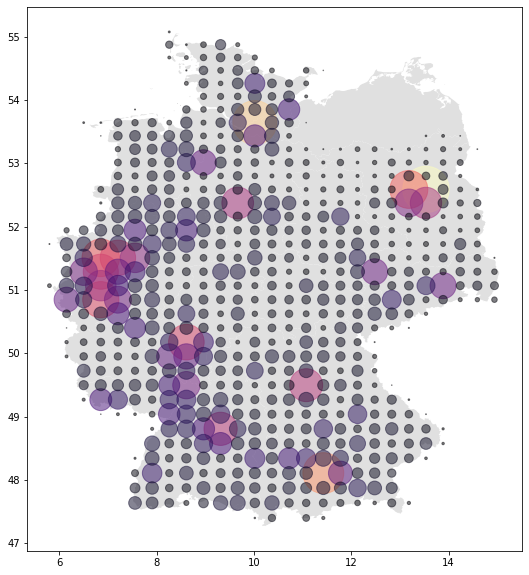
geotile_grid aggregation

Here is an example using geopandas. It extends the pandas.DataFrame with the geopandas.GeoDataFrame class.

The GeoDataFrame will pick the "geometry" column from a DataFrame by default. The values must be shapely geometries.

from shapely.geometry import Point
import geopandas
import matplotlib.pyplot as plt
import matplotlib.colors

from elastipy import Search, geotile_to_lat_lon

s = Search(index="elastipy-example-car-accidents")
agg = s.agg_geotile_grid("location", field="location", precision=10)

df = agg.execute().df()

# take hash from location column,
#   convert to latitude and longitude
#   and create a shapely.Point
#   (which expects longitude, latitude)
df["geometry"] = df.pop("location").map(
    lambda v: Point(geotile_to_lat_lon(v)[::-1])
)

# have a color for each point with matplotlib tools
cmap = plt.cm.magma
norm = matplotlib.colors.Normalize(
    df["location.doc_count"].min(), df["location.doc_count"].max()
)
df["color"] = df["location.doc_count"].map(lambda v: cmap(norm(v))[:3] + (.5,))

gdf = geopandas.GeoDataFrame(df)

fig, ax = plt.subplots(figsize=(10, 10))
# plot a shapefile from https://biogeo.ucdavis.edu/data/gadm3.6
geopandas.read_file("cache/gadm36_DEU_1.shp").plot(ax=ax, color="#e0e0e0")

gdf.plot(
    c=gdf["color"], markersize=gdf["location.doc_count"] / 3,
    aspect=1.3,
    ax=ax,
)